JUDEA PEARL

FULL-SIZE SLIDES CAN BE VIEWED BY CLICKING ON THUMB-NAILS

ALTERNATIVELY, YOU CAN OPEN A NEW WEB BROWSER AND VIEW THE TEXT AND SLIDES SIMULTANEOUSLY

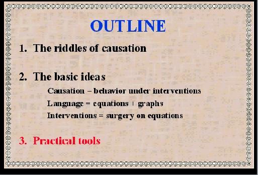
SLIDE 58: OUTLINE

Things brings us to part-3 of the lecture, where I will demonstrate how the ideas presented thus far can be used to solve new problems of practical importance.

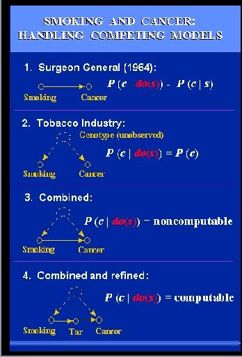
SLIDE 59: DOES SMOKING CAUSE CANCER

Consider the century old debate concerning the effect of smoking on lung cancer. In 1964, the Surgeon General issued a report linking cigarette smoking to death, cancer and most particularly, lung cancer. The report was based on non-experimental studies, in which a strong correlation was found between smoking and lung cancer, and the claim was that the correlation found is causal, namely: If we ban smoking, the rate of cancer cases will be roughly the same as the one we find today among non-smokers in the population. These studies came under severe attacks from the tobacco industry, backed by some very prominent statisticians, among them Sir Ronald Fisher. The claim was that the observed correlations can also be explained by a model in which there is no causal connection between smoking and lung cancer. Instead, an unobserved genotype might exist which simultaneously

This is all history. Now we enter a hypothetical era where representatives of both sides decide to meet and iron out their differences. The tobacco industry concedes that there might be some weak causal link between smoking and cancer and representatives of the health group concede that there might be some weak links to genetic factors. Accordingly, they draw this combined model, and the question boils down to assessing, from the data, the strengths of the various links. They submit the query to a statistician and the answer comes back immediately: IMPOSSIBLE. Meaning: there is no way to estimate the strength from the data, because any data whatsoever can perfectly fit either one of these two extreme models. So they give up, and decide to continue the political battle as usual.

Before parting, a suggestion comes up: perhaps we can resolve our differences, if we measure some auxiliary factors, For example, since the causal link model is based on the understanding that smoking affects lung cancer through the accumulation of tar deposits in the lungs, perhaps we can measure the amount of tar deposits in the lungs of sampled individuals, and this might provide the necessary information for quantifying the links? Both sides agree that this is a reasonable suggestion, so they submit a new query to the statistician: Can we find the effect of smoking on cancer assuming that an intermediate measurement of tar deposits is available??? The statistician comes back with good news: IT IS COMPUTABLE and, moreover, the solution is given in close mathematical form. HOW?

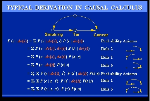
SLIDE 60: TYPICAL DERIVATION IN CAUSAL CALCULUS

The statistician receives the problem, and treats it as a problem in High School ALGEBRA: We need to compute P(cancer) under hypothetical action, from non-experimental data, namely, from expressions involving NO ACTIONS. Or: we need to eliminate the "do" symbol from the initial expression. The elimination proceeds like ordinary solution of algebraic equation - in each stage, a new rule is applied, licensed by some subgraph of the diagram, until eventually leading to a formula involving only WHITE SYMBOLS, meaning expression computable from non-experimental data. You are probably wondering whether this derivation solves the smoking-cancer debate. The answer is NO. Even if we could get the data on tar deposits, the model above is

quite simplistic, as it is based on certain assumptions which both parties might not agree to. For instance, that there is no direct link between smoking and lung cancer, immediated by tar deposits. The model would need to be refined then, and we might end up with a graph containing 20 variables or more. There is no need to panic when someone tells us: "you did not take this or that factor into account". On the contrary, the graph welcomes such new ideas, because it is so easy to add factors and measurements into the model. Simple tests are now available that permit an investigator to merely glance at the graph and decide if we can compute the effect of one variable on another.

Our next example illustrates how a long-standing problem is solved by purely graphical means - proven by the new algebra. The problem is called THE ADJUSTMENT PROBLEM or "the covariate selection problem" and represents the practical side of Simpson's paradox.

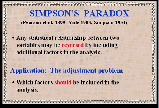
SLIDE 61: SIMPSON'S PARADOX

Simpson's paradox, first noticed by Karl Pearson in 1899, concerns the disturbing observation that every statistical relationship between two variables may be REVERSED by including additional factors in the analysis. For example, you might run a study and find that students who smoke get higher grades, however, if you adjust for AGE, the opposite is true in every AGE GROUP, namely, smoking predicts lower grades. If you further adjust for PARENT INCOME, you find that smoking predicts higher grades again, in every AGE-INCOME group, and so on. Equally disturbing is the fact that no one has been able to tell us which factors SHOULD be included in the analysis. Such factors can now be identified by simple graphical means.

The classical case demonstrating Simpson's paradox took place in 1975, when UC Berkeley was investigated for sex bias in graduate admission. In this study, overall data showed a higher rate of admission among male applicants, but, broken down by departments, data showed a slight bias in favor of admitting female applicants. The explanation is simple: female applicants tended to apply to more competitive departments than males, and in these departments, the rate of admission was low for both males and females.

SLIDE 62: FISHNET

To illustrate this point, imagine a fishing boat with two different nets, a large mesh and a small net. A school of fish swim towards the boat and seek to pass it. The female fish try for the small-mesh challenge, while the male fish try for the easy route. The males go through and only females are caught. Judging by the final catch, preference toward female is clearly evident. However, if analyzed separately, each individual net would surely trap males more easily than females. Another example involves a controversy called "reverse regression", which occupied the social science literature in the 1970's. Should we, in salary discrimination cases, compare salaries of equally qualified men and women, or, instead, compare qualifications of equally paid men and women? Remarkably, the two choices led to

opposite conclusions. It turned out that men earned a higher salary than equally qualified women, and SIMULTANEOUSLY, men were more qualified than equally paid women. The moral is that all conclusions are extremely sensitive to which variables we choose to hold constant when we are comparing, and that is why the adjustment problem is so critical in the analysis of observational studies.

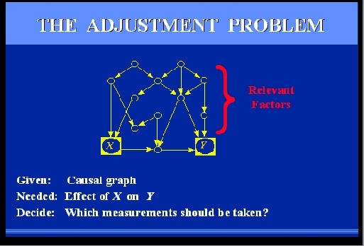
SLIDE 63: THE STATISTICAL ADJUSTMENT PROBLEM

Consider an observational study where we wish to find the effect of X on Y, for example, treatment on response. We can think of many factors that are relevant to the problem; some are affected by the treatment, some are affecting the treatment and some are affecting both treatment and response. Some of these factors may be unmeasurable, such as genetic trait or life style, others are measurable, such as gender, age, and salary level. Our problem is to select a subset of these factors for measurement and adjustment, namely, that if we compare subjects under the same value of those measurements and average, we get the right result.

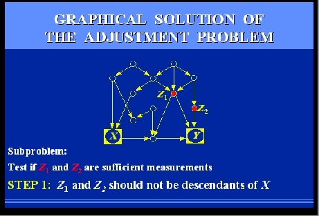
SLIDE 64: GRAPHICAL SOLUTION OF THE ADJUSTMENT PROBLEM

Let us follow together the steps that would be required to test if two candidate measurements, Z1 and Z2, would be sufficient. The steps are rather simple, and can be performed manually, even on large graphs. However, to give you the feel of their mechanizability, I will go through them rather quickly. Here we go.

SLIDES 65-69: GRAPHICAL SOLUTION OF THE ADJUSTMENT PROBLEM (CONT)

SLIDE 70: ABACUS

What I have presented to you today is a sort of pocket calculator, an ABACUS, to help us investigate certain problems of cause and effect with mathematical precision. This does not solve all the problems of causality, but the power of SYMBOLS and mathematics should not be underestimated.

SLIDE 71: A CONTEST BETWEEN THE OLD AND THE NEW ARITHMETIC

Many scientific discoveries have been delayed over the centuries for the lack of a mathematical language that can amplify ideas and let scientists communicate results. And I am convinced that many discoveries have been delayed in our century for lack of a mathematical language that can handle causation. For example, I am sure that Karl Pearson could have thought up the idea of RANDOMIZED EXPERIMENT in 1901, if he had allowed causal diagrams into his mathematics. But the really challenging problems are still ahead: We still do not have a causal understanding of POVERTY and CANCER and INTOLERANCE, and only the accumulation of data and the insight of great minds will eventually lead to such understanding. The data is all over the place, the insight is yours, and now an abacus is at your disposal too. I hope the combination amplifies each of these components. Thank you.

Remarks: technical details can be found in